This article provides examples of how to use EJAM in RStudio, especially how to use more specialized functions to find specific places to analyze, such as EPA-regulated facilities defined in various ways, and how to explore the results in more detail than the web app can provide.
Running a Basic Analysis
ejamapp()launches the web app locally (to run in RStudio on a single computer rather than on a server)ejamit()provides most results in just one function (if you already have a list of places to analyze), as shown in the Basics - Quick Start Guide
Tools for Exploring Results
For a standard analysis, the basic tools like
ejam2report(), ejam2excel(),
ejam2map(), etc. let you explore results, as shown in the
Basics - Quick Start Guide.
If you want more ways to visualize and dig into results, examples are provided below in the sections on EXPLORING RESULTS and VISUALIZATION OF FINDINGS (PLOTS). For example, you can check which groups or which facilities have notable findings.
Tools for Selecting Locations to Analyze
EJAM offers a variety of ways to specify the places to be analyzed and compared. The web app helps you select locations in several ways, including uploading a table of points, selecting facilities by industry category or ID, uploading shapefiles or lists of FIPS codes, and clicking on a map to specify one or more points.
If you are working in RStudio, and you already have identified the
points or areas to analyze, the ejamit() function will
accept 1) point coordinates, 2) a shapefile, or 3) a list of FIPS
codes.
However, if you first need to get the points (lat, lon values), or you need a more in-depth, custom approach to finding facilities or Census places to analyze, there are several groups of functions to help with that, as shown in all the examples below. They are also shown in the EJAM package reference manual, by category.
You can specify locations for analysis in a variety of ways:
Near each point: Analyze residents & the area NEAR EACH POINT (PROXIMITY ANALYSIS)
-
Facilities by ID can be defined
-
Facilities by Type can be defined
Within each polygon: Specify areas of any size and shape to analyze residents within each polygon/zone/area (based on shapefiles or Census FIPS codes)
within areas or zones on a map if you have GIS data in SHAPEFILES - Polygons (from shapefiles) could for example define redlining zones, higher risk areas based on modeling, etc.
within Census units like cities or Counties defined using FIPS CODES - Census Units such as Counties or other types of Census Units are defined by FIPS code (e.g., Counties in one State).
NEAR EACH POINT (PROXIMITY ANALYSIS)
Latitude and Longitude
You can define locations as all residents within X miles of any one or more of the specified points, and you can define those points in a few ways. One way is to upload a table of coordinates – latitude and longitude for each point, one row per site, with columns called lat and lon (or some synonyms that work). In the web app you can also pick points without a file by choosing “Click or draw on map” and clicking the map to add one or more points (click a point’s marker again to remove it).
There are also more detailed functions for working with latlon coordinates.
The simplest way to do that in the RStudio console is something like
x <- ejamit(), which prompts you to upload a spreadsheet
with lat lon columns, and asks you for the radius.
As explained below, you can get the latitudes and longitudes of
EPA-regulated facilities if you want to specify a set of facilities by
uploading their Registry ID numbers in a table, or using other
identifiers. For example, there is a function
latlon_from_programid() in the examples below.
You can also get coordinates in a few other ways, such as by NAICS (or SIC) industry names or codes, EPA program covering the set of facilities (e.g., all greenhouse gas reporters), or a Clean Air Act MACT subpart.
Facilities by ID
EPA-regulated facilities can be found in the Facility Registry Services by identification number.
See a list of functions related to EPA IDs
by Facility, using EPA Registry ID
# note frs_from_regid() and latlon_from_regid() require the frs dataset, which they try to load on demand.

frs_from_regid(testinput_registry_id[1:2])
frs_from_regid(testinput_regid)

## upload file with table of REGISTRY_ID values
testdata("regi", quiet = T) # to see sample files available with package
x1 <- latlon_from_regid(
  read_csv_or_xl(testdata("testinput_registry_id_8.xlsx", quiet = TRUE))$REGISTRY_ID
  )

## interactively upload your own file with table of REGISTRY_ID values
## (must specify the right column name)
x2 <- latlon_from_regid(read_csv_or_xl()$REGISTRY_ID)

## and run regids through EJAM
y <- ejamit(x1, radius = 1)
by Facility, using EPA Program System ID
# latlon_from_programid() requires access to the frs_by_programid dataset, which it tries to load on demand if necessary.

if (exists("frs_by_programid")) {
  latlon_from_programid(
    testinput_program_sys_id$program[1:2],
    testinput_program_sys_id$pgm_sys_id[1:2]
  )
}
#> Key: <pgm_sys_id, program, REGISTRY_ID>
#>         lat        lon  REGISTRY_ID        PGM_SYS_ACRNMS  program   pgm_sys_id
#>       <num>      <num>       <char>                <char>   <char>       <char>
#> 1: 42.89709  -71.46442 110071943048       NPDES:01R10I002    NPDES    01R10I002
#> 2: 60.53939 -145.74107 110006863153 RCRAINFO:AK0000000323 RCRAINFO AK0000000323
Facilities by Type
See a list of functions related to type of facility (NAICS/SIC/Program/MACT)
by Industry (NAICS)
You can specify sites by NAICS, but it is important to note the FRS lacks NAICS info for many regulated facilities!
naics_from_any("paint and coating", children = T)
#>      code     n2     n3     n4     n5     n6                            name
#>     <num> <char> <char> <char> <char> <char>                          <char>
#> 1:  32551     32    325   3255  32551  32551 Paint and Coating Manufacturing
#> 2: 325510     32    325   3255  32551 325510 Paint and Coating Manufacturing
#> 3: 325510     32    325   3255  32551 325510 Paint and Coating Manufacturing
#>                                    num_name
#>                                      <char>
#> 1:  32551 - Paint and Coating Manufacturing
#> 2: 325510 - Paint and Coating Manufacturing
#> 3: 325510 - Paint and Coating Manufacturing
## note latlon_from_naics() requires the frs_by_naics dataset, which it tries to load on demand.
# head(latlon_from_naics(325510))
# has about 1,000 facilities
#
# All sectors with this phrase in their NAICS title
#
#  x <- ejamit(frs_from_naics("paint and coating"), 1)}
See many more examples of Working with NAICS Codes (Industry Codes), in a section below.
by EPA Regulatory Program
See a list of functions related to EPA programs
# note latlon_from_programid() requires the frs and frs_by_programid datasets, which it tries to load on demand.
if (exists("frs_by_programid") && exists("frs")) {

  ## Map of over 10,000 facilities in FRS identified as in the E-Grid power plant database

  pts <- latlon_from_program("EGRID")[, 1:4]
  mapfast(pts)

  ## In just 1 State
  pts[, ST := state_from_latlon(lat = lat, lon = lon)$ST]
  mapfast(pts[ST == "TX", ], radius = 1)

  ## Largest lists

  epa_programs_counts <- frs_by_programid[, .N, by = "program"][order(N), ]
  epa_programs_counts[order(-N), ][1:25, ]
}
#>           program      N
#>            <char>  <int>
#>  1:      RCRAINFO 823117
#>  2:         NPDES 471051
#>  3:      NJ-NJEMS 243102
#>  4: CA-ENVIROVIEW 203747
#>  5:          ICIS 167327
#>  6:      MN-TEMPO 149471
#>  7:           AIR 134144
#>  8:           EIS 124208
#>  9:           FIS 122104
#> 10:   TX-TCEQ ACR 107572
#> 11:      AIRS/AFS  95250
#> 12:      OSHA-OIS  83729
#> 13:          SFDW  70602
#> 14:          NCDB  70163
#> 15:          ACES  63593
#> 16:       WA-FSIS  51448
#> 17:      IDNR_EFD  45827
#> 18:         ACRES  42793
#> 19:        OR-DEQ  42489
#> 20:      IN-TEMPO  39495
#> 21:          TRIS  35420
#> 22:       AZURITE  34862
#> 23:      MA-EPICS  33970
#> 24:       OH-CORE  33809
#> 25:       CA-CERS  31962
#>           program      N
#>            <char>  <int>
by MACT Subpart (hazardous air pollutant source category)
Functions related to MACT codes
# note latlon_from_mactsubpart() requires the frs_by_mact dataset, which it tries to load on demand
if (exists("frs_by_mact")) {

  # Search by name of category
  mact_table[grepl("ethylene", mact_table$title, ignore.case = T), ]
  eto <- rbind(
    latlon_from_mactsubpart("O" ),
    latlon_from_mactsubpart("WWWWW")
  )
  #  Map the category
  mapfast(eto)


  # Browse the full list of categories
  # mact_table[ , c("N", "subpart", "title")]

  # The 10 largest categories
  tail(mact_table[order(mact_table$N), c("N", "subpart", "title")], 10)

  # Many facilities lack latitude longitude information in this database
  nrow(latlon_from_mactsubpart("A", include_if_no_latlon = TRUE))
  nrow(latlon_from_mactsubpart("A", include_if_no_latlon = FALSE))

  head(latlon_from_mactsubpart("OOOO"), 2)
}
#> Key: <subpart, programid>
#>     programid subpart
#>        <char>  <char>
#> 1: 0500100022    OOOO
#> 2: 06111R9011    OOOO
#>                                                         title
#>                                                        <char>
#> 1: PRINTING, COATING AND DYEING OF FABRICS AND OTHER TEXTILES
#> 2: PRINTING, COATING AND DYEING OF FABRICS AND OTHER TEXTILES
#>                                                       dropdown_label      lat
#>                                                               <char>    <num>
#> 1: OOOO - Printing, Coating And Dyeing Of Fabrics And Other Textiles 34.27496
#> 2: OOOO - Printing, Coating And Dyeing Of Fabrics And Other Textiles 34.22082
#>           lon  REGISTRY_ID      PGM_SYS_ACRNMS  program
#>         <num>       <char>              <char>   <char>
#> 1:  -91.34179 110025082924 AIRS/AFS:0500100022 AIRS/AFS
#> 2: -119.02272 110043415578 AIRS/AFS:06111R9011 AIRS/AFS
Working with NAICS Codes (Industry Codes)
NAICS Codes to Map or Analyze Facilities in one Industrial Sector
Overview of NAICS / industry categories, at n-digit level
# see NAICS categories at the top (2-digit) level

naics_categories()

# see NAICS categories at the 3-digit level

# sorted alphabetical
naics_from_any(naics_categories(3))[order(name),.(name,code)][1:10,]
# sorted by code
naics_from_any(naics_categories(3))[order(code),.(code,name)][1:10,]
Find NAICS codes, from the name of an industry
naics_from_any('paint')Find industry names, from the NAICS codes
# get name from one code
naics_from_code(336)$name

# get the name from each code
naics_from_code(mycode)$name
Count facilities by NAICS code
mycode = c(33611, 336111, 336112)

# see counts of facilities by code (parent) and subcategories (children)
naics_counts[NAICS %in% mycode, ]

# see parent codes that contain each code
naicstable[code %in% mycode, ]
Find facilities, by name of industry
# See a data table of facilities in one industry
dataload_dynamic("frs")
#> Loading specified arrow datasets: frs
#> ✅ Token is valid!
#> Arrow-format datasets (blocks, etc.) are up-to-date -- locally-installed and package-compatible data repository versions match.
#> looking for frs in memory...
#> NULL
# if (exists("frs")) {
  industryword <- "pulp"

  head( frs_from_naics(naics_from_any(industryword)$code)[,1:4] )
#> Key: <REGISTRY_ID>
#>         lat       lon  REGISTRY_ID                       PRIMARY_NAME
#>       <num>     <num>       <char>                             <char>
#> 1: 42.60008 -72.37838 110000308612                 ERVING PAPER MILLS
#> 2: 42.61366 -71.63378 110000308881               HOLLINGSWORTH & VOSE
#> 3: 42.74216 -73.69249 110000324426       LYDALLTHERMAL/ACOUSTICAL INC
#> 4: 43.97535 -75.90653 110000325988          KNOWLTON TECHNOLOGIES LLC
#> 5: 44.22767 -74.99753 110000326120 NEWTON FALLS LAND RECLAMATION, LLC
#> 6: 41.49085 -78.67752 110000330400   DOMTAR PAPER CO/JOHNSONBURG MILL
# }
Quick map of EPA-regulated facilities in one industrial category, which you can click on to see popup windows about sites.
# note frs_from_naics() requires the frs dataset
# frs_from_naics() is slow the 1st time if it has not yet loaded the frs dataset
if (!exists("frs_arrow")) { # a more efficient format
  dataload_dynamic("frs", return_data_table = FALSE, silent = TRUE)
}

mapfast(frs_from_naics("smelt"))
(but note that this FRS dataset lacks NAICS for most facilities!)
Table of facilities in an industry, plus links to each facility in ECHO and EJSCREEN
industryword <- "chemical manuf"
#  industryword <- "smelt"
# if (exists("frs") && exists("frs_by_naics")) {
  mysites <- frs_from_naics(industryword, children = FALSE)[,1:5]

  regids <- mysites$REGISTRY_ID
  link1 <- url_echo_facility(regid = regids, as_html = T)
  link2 <- url_ejamapi(sitepoints = mysites, radius = 3, as_html = T)
  link3 <- url_ejscreenmap(lat = mysites$lat, lon = mysites$lon,  as_html = T)
  # # same:
  # my_industry <- naics_from_any("chemical manuf",children = F)[,.(code,name)]
  # mysites <- frs_from_naics(my_industry$code)[,1:5]
  mysites <- cbind(`ECHO report` = link1,
                   `EJSCREEN Report` = link2, `EJSCREEN Map` = link3,
                   mysites)
  caption = paste0(nrow(mysites), ' sites have NAICS matching "', industryword, '"')
  if (nrow(mysites) > 1500) {mysites <- mysites[1:1500, ]} # >2k rows is too much for client-side DataTables
  cat(caption,'\n')

  print(
    DT::datatable(
      mysites[1:5, ],
      escape = FALSE,     rownames = FALSE,
      caption = caption,
      filter = "top"
    )
  )
# }
Here url_ejamapi() builds links to EJSCREEN-style
community reports from the hosted EJAM API, and
url_ejscreenmap() builds deep links that open each place on
the EJSCREEN map. See the Using the EJAM API
article and ?url_ejamapi / ?url_ejscreenmap
for the full options (multisite reports, radius, combined links, and the
EJSCREEN “Send to EJAM” hand-off).
Map of facilities in an industry, plus popups with links to each facility in ECHO and EJSCREEN
mapfast(mysites)Facilities searches using industry codes or text in industry names
naics_from_any("plastics and rubber")
#>     code     n2     n3     n4     n5     n6
#>    <num> <char> <char> <char> <char> <char>
#> 1:   326     32    326    326    326    326
#>                                          name
#>                                        <char>
#> 1: Plastics and Rubber Products Manufacturing
#>                                            num_name
#>                                              <char>
#> 1: 326 - Plastics and Rubber Products Manufacturing

naics_from_any(326)
#>     code     n2     n3     n4     n5     n6
#>    <num> <char> <char> <char> <char> <char>
#> 1:   326     32    326    326    326    326
#>                                          name
#>                                        <char>
#> 1: Plastics and Rubber Products Manufacturing
#>                                            num_name
#>                                              <char>
#> 1: 326 - Plastics and Rubber Products Manufacturing

head(naics_from_any(326, children = T)[,.(code,name)])
#>      code
#>     <num>
#> 1:    326
#> 2:   3261
#> 3:  32611
#> 4: 326111
#> 5: 326112
#> 6: 326113
#>                                                                         name
#>                                                                       <char>
#> 1:                                Plastics and Rubber Products Manufacturing
#> 2:                                            Plastics Product Manufacturing
#> 3: Plastics Packaging Materials and Unlaminated Film and Sheet Manufacturing
#> 4:                                      Plastics Bag and Pouch Manufacturing
#> 5:     Plastics Packaging Film and Sheet (including Laminated) Manufacturing
#> 6:      Unlaminated Plastics Film and Sheet (except Packaging) Manufacturing

naics_from_any("pig")
#>      code     n2     n3     n4     n5     n6
#>     <num> <char> <char> <char> <char> <char>
#> 1:   1122     11    112   1122   1122   1122
#> 2:  11221     11    112   1122  11221  11221
#> 3: 112210     11    112   1122  11221 112210
#> 4:  32513     32    325   3251  32513  32513
#> 5: 325130     32    325   3251  32513 325130
#>                                       name
#>                                     <char>
#> 1:                     Hog and Pig Farming
#> 2:                     Hog and Pig Farming
#> 3:                     Hog and Pig Farming
#> 4: Synthetic Dye and Pigment Manufacturing
#> 5: Synthetic Dye and Pigment Manufacturing
#>                                            num_name
#>                                              <char>
#> 1:                       1122 - Hog and Pig Farming
#> 2:                      11221 - Hog and Pig Farming
#> 3:                     112210 - Hog and Pig Farming
#> 4:  32513 - Synthetic Dye and Pigment Manufacturing
#> 5: 325130 - Synthetic Dye and Pigment Manufacturing
naics_from_any("pig ") # space after g
#>      code     n2     n3     n4     n5     n6                name
#>     <num> <char> <char> <char> <char> <char>              <char>
#> 1:   1122     11    112   1122   1122   1122 Hog and Pig Farming
#> 2:  11221     11    112   1122  11221  11221 Hog and Pig Farming
#> 3: 112210     11    112   1122  11221 112210 Hog and Pig Farming
#>                        num_name
#>                          <char>
#> 1:   1122 - Hog and Pig Farming
#> 2:  11221 - Hog and Pig Farming
#> 3: 112210 - Hog and Pig Farming

# a OR b,  a AND b,  etc.
a = naics_from_any("plastics")

b = naics_from_any("rubber")

library(data.table)
#>
#> Attaching package: 'data.table'
#> The following object is masked from 'package:base':
#>
#>     %notin%
data.table::fintersect(a,b)[,.(name,code)] #  a AND b
#>                                                   name   code
#>                                                 <char>  <num>
#> 1:          Plastics and Rubber Products Manufacturing    326
#> 2: Rubber and Plastics Hoses and Belting Manufacturing  32622
#> 3: Rubber and Plastics Hoses and Belting Manufacturing 326220

head(data.table::funion(a,b)[,.(name,code)])     #  a OR  b
#>                                                                         name
#>                                                                       <char>
#> 1:                                 Plastics Material and Resin Manufacturing
#> 2:                                Plastics and Rubber Products Manufacturing
#> 3:                                            Plastics Product Manufacturing
#> 4: Plastics Packaging Materials and Unlaminated Film and Sheet Manufacturing
#> 5:                                      Plastics Bag and Pouch Manufacturing
#> 6:     Plastics Packaging Film and Sheet (including Laminated) Manufacturing
#>      code
#>     <num>
#> 1: 325211
#> 2:    326
#> 3:   3261
#> 4:  32611
#> 5: 326111
#> 6: 326112

# naics_subcodes_from_code(funion(a,b)[,code])[,.(name,code)]   #  plus children

head(naics_from_any(funion(a,b)[,code], children = T)[,.(name,code)] ) #  same
#>                                                                         name
#>                                                                       <char>
#> 1:                                Plastics and Rubber Products Manufacturing
#> 2:                                            Plastics Product Manufacturing
#> 3: Plastics Packaging Materials and Unlaminated Film and Sheet Manufacturing
#> 4:                                      Plastics Bag and Pouch Manufacturing
#> 5:     Plastics Packaging Film and Sheet (including Laminated) Manufacturing
#> 6:      Unlaminated Plastics Film and Sheet (except Packaging) Manufacturing
#>      code
#>     <num>
#> 1:    326
#> 2:   3261
#> 3:  32611
#> 4: 326111
#> 5: 326112
#> 6: 326113
A NAICS code can have many “children” or subcategories under it
dataload_dynamic(c("frs", "frs_by_naics"))
#> Loading specified arrow datasets: frs, frs_by_naics
#> ✅ Token is valid!
#> Arrow-format datasets (blocks, etc.) are up-to-date -- locally-installed and package-compatible data repository versions match.
#> looking for frs, frs_by_naics in memory...
#> NULL
if (exists("frs") & exists("frs_from_naics")) {

  NROW(naics_from_any("chem"))
  # about 20
  NROW(naics_from_any("chem", children = T))
  # >100
  NROW(frs_from_naics(naics_from_any("chem")$code))
  # a few thousand
  NROW(frs_from_naics(naics_from_any("chem", children = T)$code))
  # >10,000
}
#> [1] 16846
SHAPEFILES
Polygons in shapefiles as the places to compare
You can upload polygons in a shapefile, and use EJAM to analyze them. See the Shiny app.
See shapefile_from_any() and other shapefile-related
functions:
shapefile_from_any()

shapefile_from_sitepoints()
shape_buffered_from_shapefile()
shape_buffered_from_shapefile_points()

shp1 <- shapefile_from_any(system.file("testdata/shapes/portland.gdb.zip", package = "EJAM"))
FIPS CODES
Counties as the places to compare
You can compare places defined by FIPS code, such as a group of US Counties.
See a list of functions for working with Census FIPS codes.
Compare all Counties in a State, using EJAM indicators
# Get FIPS of each county in Delaware
mystate <- "Delaware"
cfips <- fips_counties_from_statename(mystate)

## You could launch a web browser tab for each of the counties,
##  to see County reports like this:
#
# sapply(url_county_health(fips = cfips), browseURL)

## Analyze EJ stats for each county in the State

x <- ejamit(fips = cfips) # radius not used
DT::datatable(x$results_bysite, escape = F)

ejam2table_tall(x)

t(x$results_bysite[ , c(
  'ejam_uniq_id', 'pop', names_d_subgroups_ratio_to_state_avg), with = F])

mapfastej_counties(x$results_bysite)

cnames <- fips2countyname(x$results_bysite$ejam_uniq_id)
#cnames <- c("Kent County", "New Castle County", "Sussex County")
#cnames <- gsub(" County", "", cnames)

barplot(x$results_bysite$pctlowinc, names.arg = cnames,
        main = paste0('% Low Income by County in ', mystate))

# Another example
mystate <- "Maryland"
vname <- "% low income"
xmd <- ejamit(fips = fips_counties_from_statename(mystate))
ggblanket::gg_col(data = xmd$results_bysite,
                  y = pctlowinc,
                  x = ejam_uniq_id,
                  title = paste0(vname, ' by County in ', mystate),
                  y_title = vname
)

mapfastej_counties(xmd$results_bysite, 'state.pctile.pctlowinc')
EXPLORING RESULTS
See also
The most striking findings (e.g., which group is most over-represented?)
See examples above using ejam2report() but also you can
check some key findings like this:
out <- testoutput_ejamit_1000pts_1miles
bysite <- out$results_bysite
bysite <- setDF(copy(bysite))
ratio_benchmarks <- c(1.01, 1.50, 2, 3, 5, 10)
ratiodata <- bysite[, names_d_ratio_to_state_avg]

findings <- count_sites_with_n_high_scores(ratiodata, quiet = TRUE)  # long output to console !

tail(findings$text[findings$text != ""], 1) # the most extreme finding!
#> [1] "At at least 2% of these sites, 1 of the indicators is 5 times the average "More summary findings
dimnames(findings)
#> NULL
findings$text[2]
#> [1] "At at least 90% of these sites, 1 of the indicators is 1.05 times the average "
head(findings$stats[ , , 1], 15)
#>      cut
#> count 1.05   2   5  10
#>     0   99 707 977 997
#>     1  212 172  23   3
#>     2  152  61   0   0
#>     3  113  29   0   0
#>     4   91  21   0   0
#>     5   79   7   0   0
#>     6   81   2   0   0
#>     7  104   1   0   0
#>     8   68   0   0   0
#>     9    1   0   0   0
head(findings$stats[ , 1, ], 21)
#>      stat
#> count count  cum pct cum_pct
#>     0    99 1000  10     100
#>     1   212  901  21      90
#>     2   152  689  15      69
#>     3   113  537  11      54
#>     4    91  424   9      42
#>     5    79  333   8      33
#>     6    81  254   8      25
#>     7   104  173  10      17
#>     8    68   69   7       7
#>     9     1    1   0       0
x = findings$stats[ , 1, ]
x[x[, "cum_pct"] >= 50 & x[, "cum_pct"] <= 80, ]
#>      stat
#> count count cum pct cum_pct
#>     2   152 689  15      69
#>     3   113 537  11      54
findings$stats[ 1, , ]
#>       stat
#> cut    count  cum pct cum_pct
#>   1.05    99 1000  10     100
#>   2      707 1000  71     100
#>   5      977 1000  98     100
#>   10     997 1000 100     100
Local features and special areas – schools, hospitals, nonattainment areas, etc.
ejamit() also provides special summary statistics
related to the group of indicators that count features like schools
within each blockgroup, overlaps with specially-designated areas such as
nonattainment
areas, and lack of critical services like health insurance. See the
help for batch.summarize() for details.
The function ejam2areafeatures() is just a convenient
way to see the information in
ejamit()$results_summarized$flagged_areas created by
batch.summarize(), as used by ejamit(), from
the indicators in these lists:
names_featuresinareanames_flagnames_criticalservice
Summary of whether residents at the analyzed locations are more likely to have certain types of features (schools) or special areas (Tribal, nonattainment, etc.)
Table
## out1k <- ejamit(testpoints_1000, radius = 1)
out1k <- testoutput_ejamit_1000pts_1miles
ejam2areafeatures(out1k)
#>                                                    Indicator
#> 1                                                Any schools
#> 2                                      Any places of worship
#> 3                                              Any hospitals
#> 4                                    Overlapping with Tribes
#> 5                           Overlapping with Impaired Waters
#> 6                      Overlapping with Non-Attainment Areas
#> 7           Overlapping with CEJST Disadvantaged Communities
#> 8         Overlapping with EPA IRA Disadvantaged Communities
#> 9                Overlapping with Housing Burden Communities
#> 10                        Overlapping with Food Desert Areas
#> 11                   % Households without Broadband Internet
#> 12                         % People without Health Insurance
#> 13 Overlapping with Transportation Disadvantaged Communities
#>    Percent_of_these_Sites Percent_of_these_People
#> 1                    76.4                    29.4
#> 2                    75.9                    34.6
#> 3                    30.0                     5.4
#> 4                     2.7                     0.2
#> 5                    89.2                    41.0
#> 6                    57.7                    81.3
#> 7                    50.5                    40.9
#> 8                    65.5                    51.8
#> 9                    27.6                    28.1
#> 10                   50.6                    14.3
#> 11                   12.4                    10.9
#> 12                    8.3                     9.0
#> 13                   89.5                    58.8
#>    Percent_of_all_People_Nationwide ratio Percent_of_all_People_Statewide
#> 1                              31.3  0.94                            31.3
#> 2                              38.8  0.89                            30.5
#> 3                               4.6  1.17                             4.0
#> 4                               1.6  0.12                             0.8
#> 5                              56.7  0.72                            50.3
#> 6                              57.2  1.42                            75.9
#> 7                              32.3  1.27                            30.4
#> 8                              42.8  1.21                            40.5
#> 9                              12.5  2.25                            17.5
#> 10                             25.0  0.57                            18.5
#> 11                             11.5  0.95                            10.0
#> 12                              8.7  1.03                             7.5
#> 13                             69.5  0.85                            64.2
#>    ratio_to_state_avg                rname
#> 1                0.94           num_school
#> 2                1.13           num_church
#> 3                1.35         num_hospital
#> 4                0.25         yesno_tribal
#> 5                0.81      yesno_impwaters
#> 6                1.07      yesno_airnonatt
#> 7                1.35       yesno_cejstdis
#> 8                1.28         yesno_iradis
#> 9                1.61    yesno_houseburden
#> 10               0.77     yesno_fooddesert
#> 11               1.09       pctnobroadband
#> 12               1.20 pctnohealthinsurance
#> 13               0.92       yesno_transdis
Plots showing whether residents at the analyzed locations are more likely to have certain types of features or special areas
To view these special ratios, since they are not in the main table
ejamit()$results_bysite, you can reformat them for plotting
like this:
## out <- ejamit(testpoints_1000, radius = 1)
out <- testoutput_ejamit_1000pts_1miles

## simple barplot on special areas and features like schools:

ejam2barplot_areafeatures(out1k)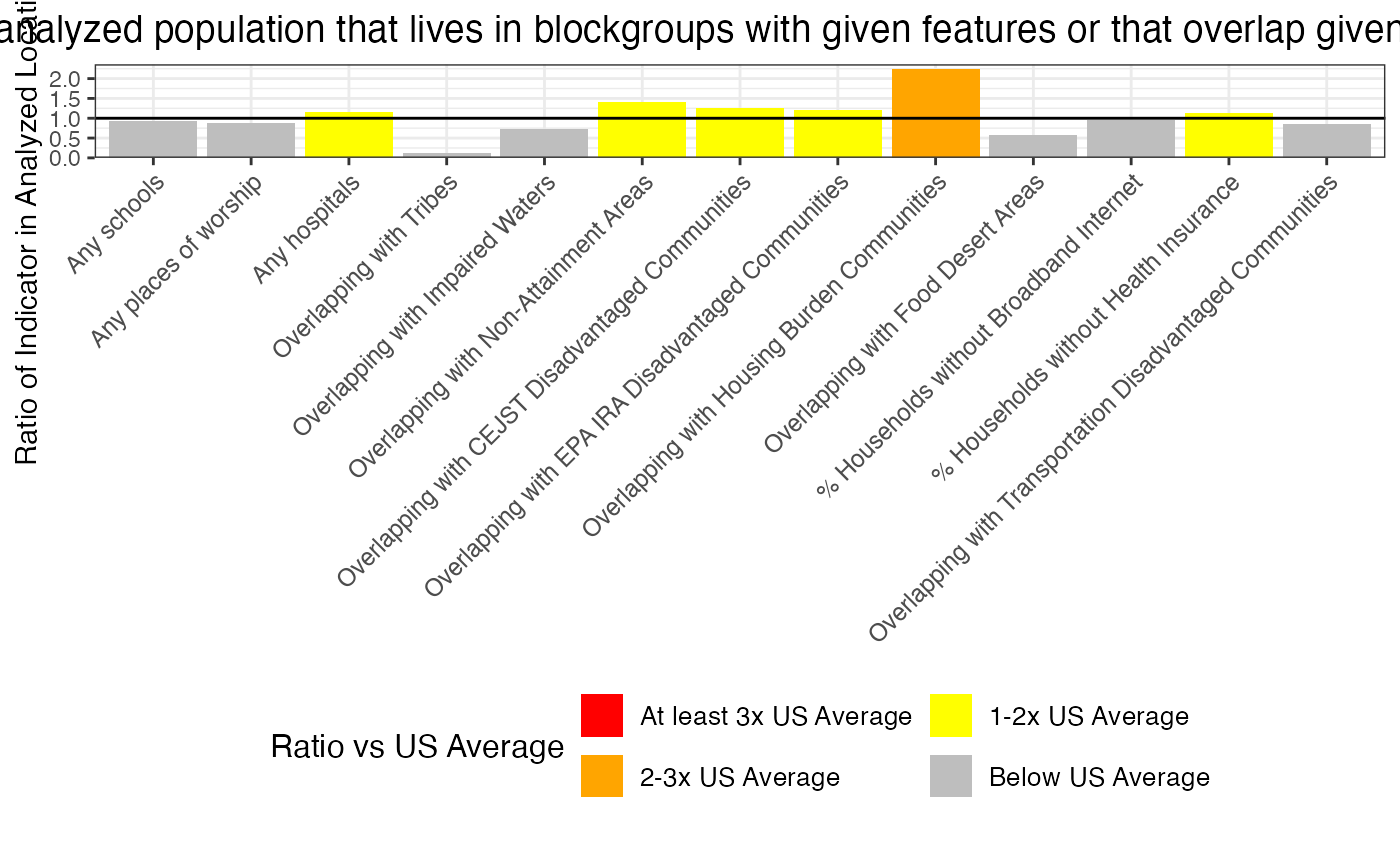
## note the sitenumber param is not supported for these statsSite by site detailed results in datatable format in RStudio viewer:
out2 <- testoutput_ejamit_100pts_1miles
DT::datatable(out2$results_bysite[1:5,   ], escape = FALSE, rownames = FALSE)

# To see all 1,000 sites in table:
#DT::datatable(out2$results_bysite[1:1000, ], escape = FALSE, rownames = FALSE)
Overall results for a few key indicators, as raw output in console:
out2 <- testoutput_ejamit_100pts_1miles

names(out2)
#> [1] "results_overall"                     "results_bysite"
#> [3] "results_bybg_people"                 "longnames"
#> [5] "count_of_blocks_near_multiple_sites" "results_summarized"
#> [7] "formatted"                           "sitetype"
cbind(overall = as.list( out2$results_overall[ , ..names_d]))
#>                  overall
#> Demog.Index      1.676867
#> Demog.Index.Supp 1.693936
#> pctlowinc        0.319063
#> pctlingiso       0.06979021
#> pctunemployed    0.06099867
#> pctlths          0.1370251
#> pctunder5        0.05797804
#> pctover64        0.144583
#> pctmin           0.5839562
cbind(overall = as.list( out2$results_overall[ , ..names_d_subgroups]))
#>                 overall
#> pcthisp         0.2524003
#> pctnhba         0.1715473
#> pctnhaa         0.1104285
#> pctnhaiana      0.003836903
#> pctnhnhpia      0.002411388
#> pctnhotheralone 0.005859968
#> pctnhmulti      0.0374718
#> pctnhwa         0.4160438
Overall results for the very long list of all indicators, as raw output in console:
out2 <- testoutput_ejamit_100pts_1miles

head(
  ejam2table_tall(out2)
  , 20)
# head(
#   cbind(as.list(out2$results_overall))
#   , 12)
Just one site, all the indicators
head(
  ejam2table_tall(out2, sitenumber = 1)
  , 20)
See indicators aggregated over all people across all sites
## view output of batch run aggregation ####
out <- testoutput_ejamit_1000pts_1miles
head(cbind(overall = as.list( out$results_overall)))
#>              overall
#> EJAM Report  "<a href="https://api.ejanalysis.com" target="_blank">EJAM Site Report</a>"
#> EJSCREEN Map "https://pedp-ejscreen.azurewebsites.net/index.html"
#> ejam_uniq_id NA
#> valid        TRUE
#> invalid_msg  ""
#> pop          8609095

## To see just some subset of indicators, like Environmental only:
cbind(overall = as.list( out$results_overall[ , ..names_e])); cat("\n")
#>                 overall
#> pm              9.585876
#> o3              66.39456
#> no2             10.83491
#> dpm             0.33535
#> rsei            4536.487
#> traffic.score   3974228
#> pctpre1960      0.4124342
#> proximity.npl   1.291201
#> proximity.rmp   0.8603396
#> proximity.tsdf  10.90486
#> ust             8.545572
#> proximity.npdes 527761.8
#> drinking        1.674242
cbind(overall = as.list( out$results_overall[ , ..names_d])); cat("\n")
#>                  overall
#> Demog.Index      1.649779
#> Demog.Index.Supp 1.666516
#> pctlowinc        0.3107655
#> pctlingiso       0.07357484
#> pctunemployed    0.06180353
#> pctlths          0.1332822
#> pctunder5        0.0575535
#> pctover64        0.1394766
#> pctmin           0.5792066
cbind(overall = as.list( out$results_overall[ , ..names_d_subgroups])); cat("\n")
#>                 overall
#> pcthisp         0.2945468
#> pctnhba         0.1434055
#> pctnhaa         0.09549668
#> pctnhaiana      0.003141675
#> pctnhnhpia      0.001910486
#> pctnhotheralone 0.005492147
#> pctnhmulti      0.0352133
#> pctnhwa         0.4207934
cbind(overall = as.list( out$results_overall[ , ..names_e_pctile])); cat("\n")
#>                        overall
#> pctile.pm              83
#> pctile.o3              76
#> pctile.no2             80
#> pctile.dpm             87
#> pctile.rsei            85
#> pctile.traffic.score   88
#> pctile.pctpre1960      68
#> pctile.proximity.npl   93
#> pctile.proximity.rmp   77
#> pctile.proximity.tsdf  91
#> pctile.ust             87
#> pctile.proximity.npdes 99
#> pctile.drinking        84
cbind(overall = as.list( out$results_overall[ , ..names_d_pctile])); cat("\n")
#>                         overall
#> pctile.Demog.Index      68
#> pctile.Demog.Index.Supp 57
#> pctile.pctlowinc        57
#> pctile.pctlingiso       81
#> pctile.pctunemployed    67
#> pctile.pctlths          69
#> pctile.pctunder5        60
#> pctile.pctover64        41
#> pctile.pctmin           70
# cbind(overall = as.list( out$results_overall[ , ..names_ej_pctile])); cat("\n")
See the US or State reference averages and percentiles
These lookup tables hold the benchmark values that site results get compared against (for example in the “Compared to US/State Averages” barplots below).
# US mean plus key percentiles, for environmental and demographic indicators
usastats_query(varnames = names_e)
#>   REGION PCTILE      pm       o3     no2    dpm         rsei traffic.score
#> 1    USA      0  3.2886  38.7784  0.0368 0.0006       0.0000          0.00
#> 2    USA      5  5.9044  51.5233  2.7216 0.0399       1.2869      11202.88
#> 3    USA     50  8.1561  60.2542  7.5653 0.1560     603.0321     814996.31
#> 4    USA     80  9.3060  67.4684 10.7127 0.2721    3121.8767    2703270.44
#> 5    USA     90 10.4548  72.5816 12.4905 0.3663    6944.4256    4437336.81
#> 6    USA     95 12.9132  77.4690 14.2645 0.4731   14174.0358    6414285.76
#> 7    USA     99 15.4726  95.3021 17.7069 0.7425   68182.1517   11202280.01
#> 8    USA    100 25.6121 112.8128 25.2692 2.9793 4512172.0810   30181802.55
#> 9    USA   mean  8.4473  61.8496  7.8464 0.1911    4611.7526    1687230.49
#>   pctpre1960 proximity.npl proximity.rmp proximity.tsdf      ust
#> 1     0.0000        0.0000        0.0000         0.0000   0.0000
#> 2     0.0000        0.0000        0.0000         0.0000   0.0000
#> 3     0.2110        0.0000        0.2693         1.2741   0.8243
#> 4     0.5893        0.3794        0.9612         5.2036   5.1726
#> 5     0.7612        0.8419        1.5360         9.4650  10.2846
#> 6     0.8585        1.5980        2.1131        16.0833  17.0185
#> 7     0.9637        7.6275        3.8023        28.7909  35.7895
#> 8     1.0000       46.0823       18.0597        82.2821 137.8717
#> 9     0.2999        0.3948        0.5703         3.5356   3.6375
#>   proximity.npdes drinking
#> 1    0.000000e+00   0.0000
#> 2    0.000000e+00   0.0000
#> 3    5.047510e+01   0.0000
#> 4    2.302532e+03   1.0000
#> 5    1.351239e+04   4.6342
#> 6    4.070759e+04  10.0000
#> 7    2.374183e+05  32.0000
#> 8    7.709095e+09 899.0000
#> 9    7.018054e+05   2.2147

# US means only, as a tidy 1-column matrix (indicators as rownames)
usastats_means(names_d)
#>                  us.avg
#> Demog.Index      1.3407
#> Demog.Index.Supp 1.6423
#> pctlowinc        0.3041
#> pctlingiso       0.0481
#> pctunemployed    0.0561
#> pctlths          0.1131
#> pctunder5        0.0539
#> pctover64        0.1779
#> pctmin           0.3958

# the same for one state: mean plus key percentiles
statestats_query("MD", varnames = names_e)
#>   REGION PCTILE    pm     o3    no2   dpm      rsei traffic.score pctpre1960
#> 1     MD      0 5.367 52.958  1.374 0.029     0.022          0.00      0.000
#> 2     MD      5 5.897 54.968  3.192 0.075    19.548      45189.41      0.000
#> 3     MD     50 6.919 60.564  7.289 0.218   258.382    1351498.75      0.215
#> 4     MD     80 7.073 62.747  9.247 0.281   667.044    2665707.04      0.653
#> 5     MD     90 7.162 62.901 10.231 0.310   951.123    3083701.81      0.835
#> 6     MD     95 7.229 62.953 12.129 0.320  1279.760    3398964.01      0.911
#> 7     MD     99 7.415 63.015 14.731 0.354  2143.295    4094602.44      1.000
#> 8     MD    100 7.662 63.058 17.136 0.615 49507.599    5150543.37      1.000
#> 9     MD   mean 6.808 60.295  7.270 0.208   432.084    1489436.75      0.321
#>   proximity.npl proximity.rmp proximity.tsdf    ust proximity.npdes drinking
#> 1         0.000         0.000          0.000  0.000           0.000    0.000
#> 2         0.000         0.000          0.000  0.000           0.008    0.000
#> 3         0.103         0.179          3.021  1.007          86.222    0.000
#> 4         0.358         0.897          7.585  3.427       11172.758    0.000
#> 5         0.612         1.735         11.380  5.129      204977.996    0.000
#> 6         0.997         2.455         14.531  6.496      766925.607    0.000
#> 7         2.876         3.174         18.700 10.689     2895564.429    1.000
#> 8        11.243         5.143         28.006 17.463    12715947.245   11.000
#> 9         0.278         0.523          4.434  1.883      137010.635    0.045

# state means as a matrix with indicators as rows and one column per state
# (ST may repeat, e.g. one entry per site)
statestats_means(ST = c("MD", "VA"), varnames = names_e[1:3])
#>          MD      VA
#> pm   6.8078  6.8280
#> o3  60.2948 53.8339
#> no2  7.2701  6.3434
VISUALIZATION OF FINDINGS (PLOTS)
See examples below, and the list of plot-related functions.
Indicators
Barplot showing which indicator is most elevated overall
out <- testoutput_ejamit_1000pts_1miles

ejam2barplot(out,
             varnames = c(names_d_ratio_to_state_avg, names_d_subgroups_ratio_to_state_avg),
             main = "Residential population group percentages at Selected Sites Compared to State Averages")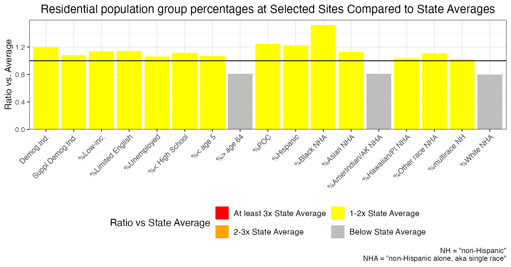
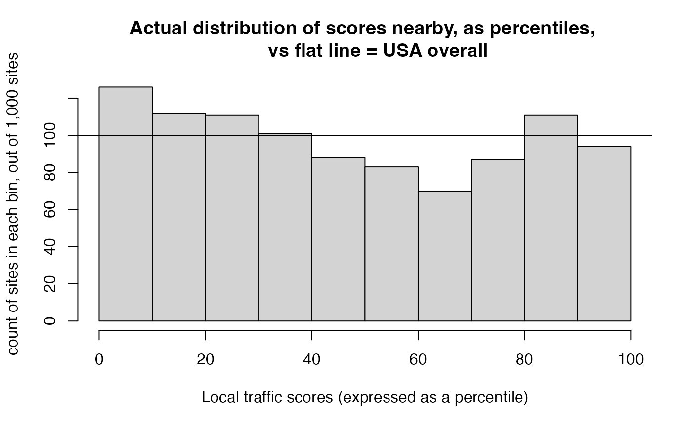
Histogram of indicators distribution over all people across all sites
hist(out$results_bysite$pctile.traffic.score, 10, xlab = "Local traffic scores (expressed as a percentile)",
     ylab = "count of sites in each bin, out of 1,000 sites", freq = TRUE,
     main = "Actual distribution of scores nearby, as percentiles,
     vs flat line = USA overall")
abline(h = nrow(out$results_bysite)/10)