
How to use EJAM to analyze zip codes
EJAM can analyze various kinds of Census-defined areas, including States, Counties, Tracts, Blockgroups, and Cities/CDPs/etc.
However, you may need to analyze zip codes.
Census uses ZIP Code Tabulation Areas (ZCTAs), which are generalized
areal representations of United States Postal Service (USPS) ZIP Code
service areas. See help("zctas", package="tigris")
Note a zip can be the same as a county fips in many cases, as with 10001!
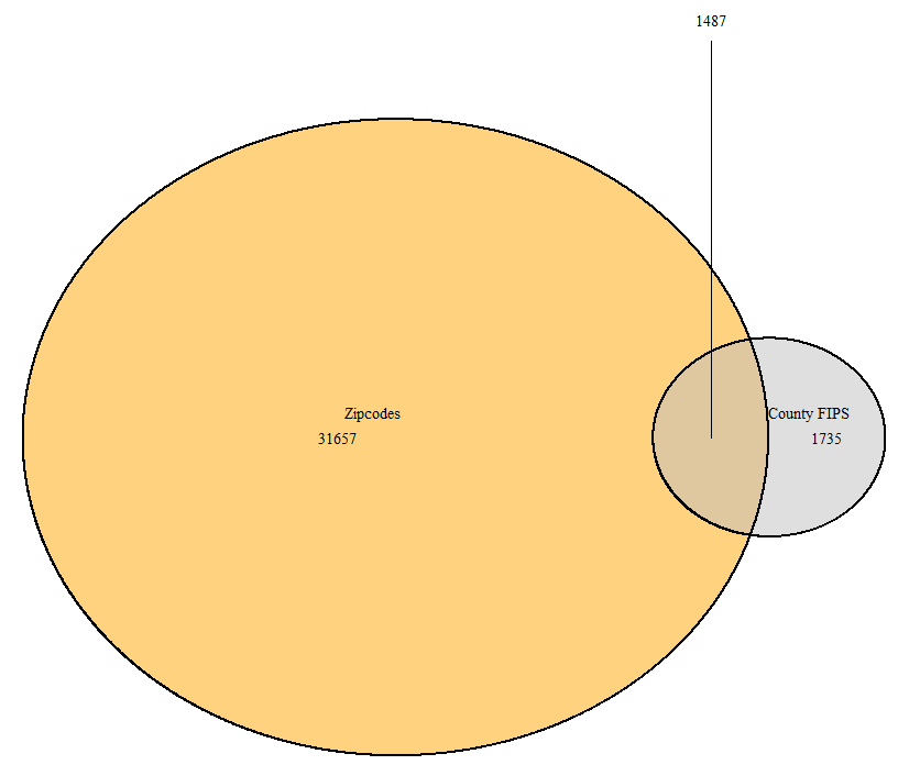
The short way: ejamit(zipcode = )
The simplest way to analyze zip codes is to pass them directly to
ejamit(), which converts them to ZCTA polygons via
shapes_from_zip() and analyzes them like any other
shapefile (the first use downloads a large national boundaries file,
which is slow, but it is cached locally so later uses are fast):
out <- ejamit(zipcode = c("10012", "10506"))

# summary report, with the places described as zip codes and their bounds mapped
ejam2report(out)

# or just get the ZCTA polygons, to map or inspect them
z <- shapes_from_zip(c("10012", "10506"))
mapfast(z)
The rest of this article shows the manual, step-by-step version of that workflow, which offers more control (e.g., other sources of zip code polygons).
Manual step-by-step approach
The original (pre-2025) EJSCREEN API did not handle zip codes. It can show where the center of the zip code is but will not map its bounds or provide a report easily via the API.
# Just see where the zipcode is, not its boundaries
# (use zip= , not wherestr= : a bare 5-digit wherestr is now read as a county FIPS first,
#  so wherestr = '10001' would open Kent County, DE instead of this Manhattan zip code)
browseURL(url_ejscreenmap(zip = '10001'))
To map and analyze zip codes you can download shapefiles for them and analyze or map them in EJAM as shown below.
downloading zcta polygons
Takes time to download!
library(tigris)
# options(tigris_use_cache=TRUE) # done by EJAM load/attach
options(tigris_refresh=FALSE)
#zcta_DE <- zctas(starts_with = fips_from_name('DE'), keep_zipped_shapefile = T) # all in the state
#zcta1 <- zctas(starts_with = c("10001"))  # one zip
zcta2 <- zctas(starts_with = c("10012", "10506"))  # two zipcodes

z = shapefile_from_any(zcta2)
mapping zcta polygons
mapfast(z)Another source of zip code polygons (esri service)
# Download spatial bounds for all zipcodes in Delaware
ST1 <- "DE"
url1 <- paste0("https://services.arcgis.com/P3ePLMYs2RVChkJx/ArcGIS/rest/services/USA_Boundaries_2022/FeatureServer/3/query?",
  "where=STATE%3D%27", ST1, "%27",
  "&geometryType=esriGeometryEnvelope&inSR=&spatialRel=esriSpatialRelIntersects&resultType=none&distance=0.0&units=esriSRUnit_Meter&relationParam=&returnGeodetic=false",
  "&outFields=*",
  "&returnGeometry=true",
  "&f=json")
require(httr2); require(sf); require(mapview)
response1 <- httr2::req_perform(httr2::request(url1))
text1 <- httr2::resp_body_string(response1)
shp1 <- sf::st_read(text1)
mapview::mapview(shp1)
see EJSCREEN map at a zip code
The EJScreen map app can be opened at zip code(s) via a deep link,
using its ?zip= launch-URL parameter – the explicit way to
pass a zip code. That matters because a bare 5-digit number is
ambiguous: 10001 is both a Manhattan zip code and Kent County, DE’s
county FIPS, and EJScreen deep links read a bare 5-digit
wherestr= as a county FIPS first (EJAM’s convention). The
zip argument of url_ejscreenmap() builds the
unambiguous zip links:
# one zip code: EJScreen opens centered there, with a pin and the site report popup
browseURL(url_ejscreenmap(zip = "20019"))
#> opens https://pedp-ejscreen.azurewebsites.net/index.html?zip=20019

# note the zip parameter, unlike wherestr, is never confused with a county FIPS:
url_ejscreenmap(zip = "10001")  # zip 10001, in Manhattan, NY
url_ejscreenmap(fips = "10001") # county FIPS 10001 = Kent County, DE (boundary drawn)

# several zips in one link (the map zooms to fit all of them),
# and radius= prefills the report buffer distance in miles:
url_ejscreenmap(zip = c("20019", "20020"), combined = TRUE, radius = 1)
#> "https://pedp-ejscreen.azurewebsites.net/index.html?zip=20019,20020&radius=1"

# a zip passed as a number gets its leading zeroes restored:
url_ejscreenmap(zip = 1001) # zip 01001, Agawam, MA
These links need the EJScreen release that added deep links (see Public-Environmental-Data-Partners/EJScreen#70); the map pins the zip’s location – for analyzing the zip code’s actual boundaries, use the zcta polygons approach above.
analyzing zip codes in EJAM
You can analyze zip codes in EJAM like this:
out = ejamit(shapefile = z, radius = 0)summary report on zipcodes
ejam2report(out,
            analysis_title = "Zip codes",
            site_method = 'SHP',
            shp = z)
compare sites
# put zip code in the x axis labels!
ejam2barplot_sites(out, names.arg = z$GEOID20, sortby = FALSE) # zcta2$GEOID20

# This table view works, but the links to reports do not work with zipcodes
ejam2tableviewer(out)
map of detailed results
out_plus_shape = sf::st_as_sf(
  data.frame(out$results_bysite, z)
  )
# put zip code in the map popups!
out_plus_shape$ejam_uniq_id = paste0(out_plus_shape$ejam_uniq_id, " (zip ", z$GEOID20, ")")
mapfastej(out_plus_shape)
Note that ejam2map() will not work for zipcodes!